Viewing Geotechnical Data in QGIS

What you'll build: A comprehensive QGIS project with your geotechnical data, styled, and ready for analysis.

You'll learn to: Transform AGS files into GeoPackage format and set up professional visualization in QGIS with proper styling and 3D capabilities.

Time needed: 30 minutes

Result: Professional maps and 3D visualizations of your ground investigation data that you can use for analysis, reporting, and stakeholder presentations.

Instead of multiple specialized files, you'll have one comprehensive geospatial database that works with QGIS and other GIS software.

You can also explore the data preparation workflow interactively in a marimo notebook in your web browser. marimo is a reactive Python notebook that automatically updates when you modify data or code. We're big fans of it here at Bedrock.

Prerequisites

Before starting, ensure you have:

• Python 3.13+ with ability to install packages (we recommend uv).
• QGIS installed on your system.
• AGS files from your geotechnical project. Download the AGS files from the demo here.
• Your project's coordinate reference system (CRS). Check your geotechnical report or survey data.
• Local development setup: Code editor and command line access.

1. Data Transformation With bedrock-ge

1.1: Set Up Your Python Environment

Create a new Python project using the uv init command. Learn more on Python projects using uv.

uv init

Install the required packages:

uv add bedrock-ge pyproj

1.2: Read AGS Files using Bedrock

First, you'll convert your AGS files to geospatial data using bedrock-ge.

For this, you need to know the horizontal and vertical Coordinate Reference System your AGS data uses. For the demo files, it's Hong Kong 1980 Grid System (EPSG:2326) and Hong Kong Principle Datum (EPSG:5738).

You'll convert each AGS file to a single database object.

from bedrock_ge.gi.ags import ags_to_brgi_db_mapping
from bedrock_ge.gi.db_operations import merge_dbs
from bedrock_ge.gi.geospatial import create_brgi_geodb
from bedrock_ge.gi.io_utils import geodf_to_df
from bedrock_ge.gi.mapper import map_to_brgi_db
from pyproj import CRS
from pathlib import Path

projected_crs = CRS("EPSG:2326")  # Hong Kong 1980 Grid System
vertical_crs = CRS("EPSG:5738")   # Hong Kong Principle Datum

Use EPSG.io to find the correct codes for your project data.

1.3: Convert AGS Files to GeoPackage

When working with multiple AGS files from the same project:

folder_path = Path("./hk_kaitak_ags_files")
ags_files = list(folder_path.glob("*AGS")) + list(folder_path.glob("*ags"))

ags_file_brgi_dbs = []

for file_path in ags_files:
    print(f"[Processing {file_path.name}]")
    brgi_mapping = ags_to_brgi_db_mapping(file_path, projected_crs, vertical_crs)
    brgi_db = map_to_brgi_db(brgi_mapping)
    ags_file_brgi_dbs.append(brgi_db)

# Merge all files into a single database
merged_brgi_db = merge_dbs(ags_file_brgi_dbs)
geodb = create_brgi_geodb(merged_brgi_db)  # Transforms to geospatial data
write_brgi_db_to_file(geodb, "combined_gi_data.gpkg", driver="GPKG")

The result is a single GeoPackage file containing all your geotechnical data with proper 3D geometries and relationships preserved.

2: Visualizing in QGIS

2.1: Open GeoPackage in QGIS

1. Launch QGIS and create a new project

2. Connect to your GeoPackage:

   • In the Browser Panel (left sidebar), right-click on GeoPackage
   • Select New Connection
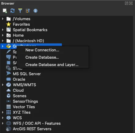
   • Browse to your .gpkg file and click Open
   • The GeoPackage will appear in the Browser Panel with a database icon

3. Explore and load tables:

   • Expand your GeoPackage connection to see all available tables

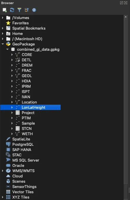
   • Key tables include:

     • LonLatHeight: Ground investigation locations in WGS84 coordinates
     • Location: Borehole locations with 3D geometry
     • InSituTests_GEOL: Geological descriptions with depth intervals
     • InSituTests_ISPT: Standard Penetration Test results
     • InSituTests_WETH: Weathering grade information

   • Load essential tables: Double-click to load both LonLatHeight and Location tables (needed for joining data)

   • Load additional test tables as needed for your analysis

2.2: Add Base Map Layer

Before styling your data, add a base map for geographic context:

1. Add OpenStreetMap layer:

   • Go to Browser Panel (usually on the left side)
   • Expand XYZ Tiles
   • Double-click OpenStreetMap to add it to your map

2. Arrange layer order:

   • In the Layers Panel, drag the OpenStreetMap layer to the bottom
   • Your borehole data layers should be above the base map
   • This ensures your investigation points are visible on top

Why Two Location Tables?

You'll notice both LonLatHeight and Location tables contain borehole locations:

• Location: Contains 3D vertical linestrings representing the full borehole geometry from ground surface to final depth
• LonLatHeight: Contains 2D points at ground level in WGS84 coordinates

Why the difference? QGIS doesn't display vertical linestrings well in 2D map views. They often appear as single points or don't render at all. The LonLatHeight points ensure your borehole locations are always visible on the map, while the Location table preserves the full 3D geometry for analysis.

Best practice: Use LonLatHeight for visualization and join data from Location for attributes.

2.3: Join Location Data to Points

To display borehole details with your location points, you'll join the Location table data to the LonLatHeight points:

1. Right-click the LonLatHeight layer in the Layers panel

2. Select Properties

3. Go to the Joins tab

4. Click the + button to add a new join

5. Configure the join:

   • Join layer: Select Location

   • Join field: location_uid

   • Target field: location_uid

   • Joined fields: Select only the fields you need:

     • HOLE_STAR (start date)
     • HOLE_FDEP (final depth)
     • HOLE_REM (remarks)
     • HOLE_TYPE (borehole type)

     

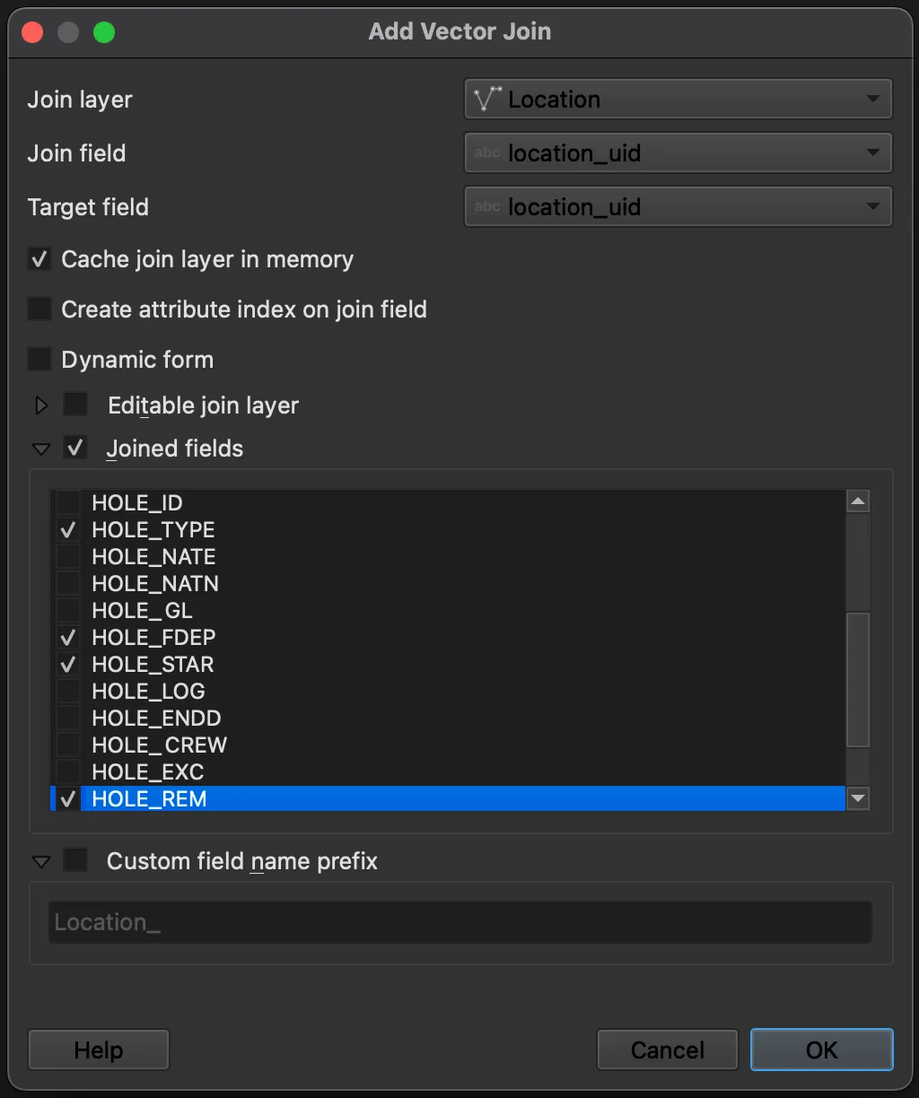
6. Click OK to apply the join

Now your LonLatHeight points have access to all the borehole details from the Location table. You can use these joined fields for styling and labeling.

2.4: Style and Explore the Data

Basic Visualization

1. Style location points by borehole type:

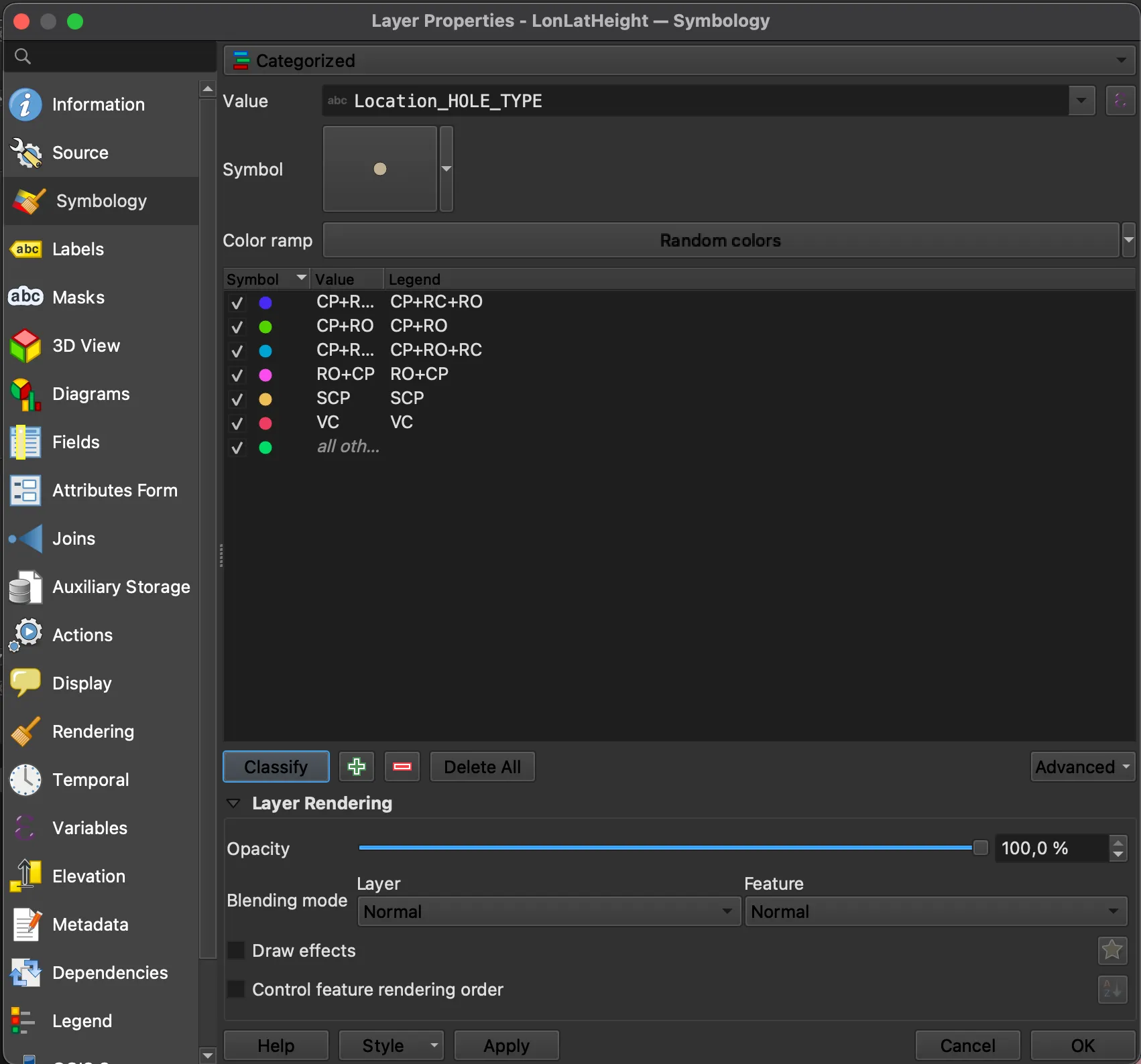
   • The LonLatHeight table displays best as points on the map

   • Right-click the layer > Properties > Symbology

   • Change from Single Symbol to Categorized

   • Set Column to Location_HOLE_TYPE to classify by borehole type

   • Click Classify

     

2. Add hole depth labels:

   • In the same Properties dialog, go to the Labels tab
   • Change from No labels to Single labels
   • Set Value to "Location_HOLE_FDEP" || 'm' to display depth with units

You should now see an overview of GI locations colored by type and with the final depth displayed.

Conclusion

With bedrock-ge, your AGS files become proper geospatial data that works with standard GIS tools like QGIS. Instead of dealing with multiple specialized formats, you have a single database that preserves all relationships between locations, tests, and results, which enables spatial analysis and easy mapping.