
Getting started
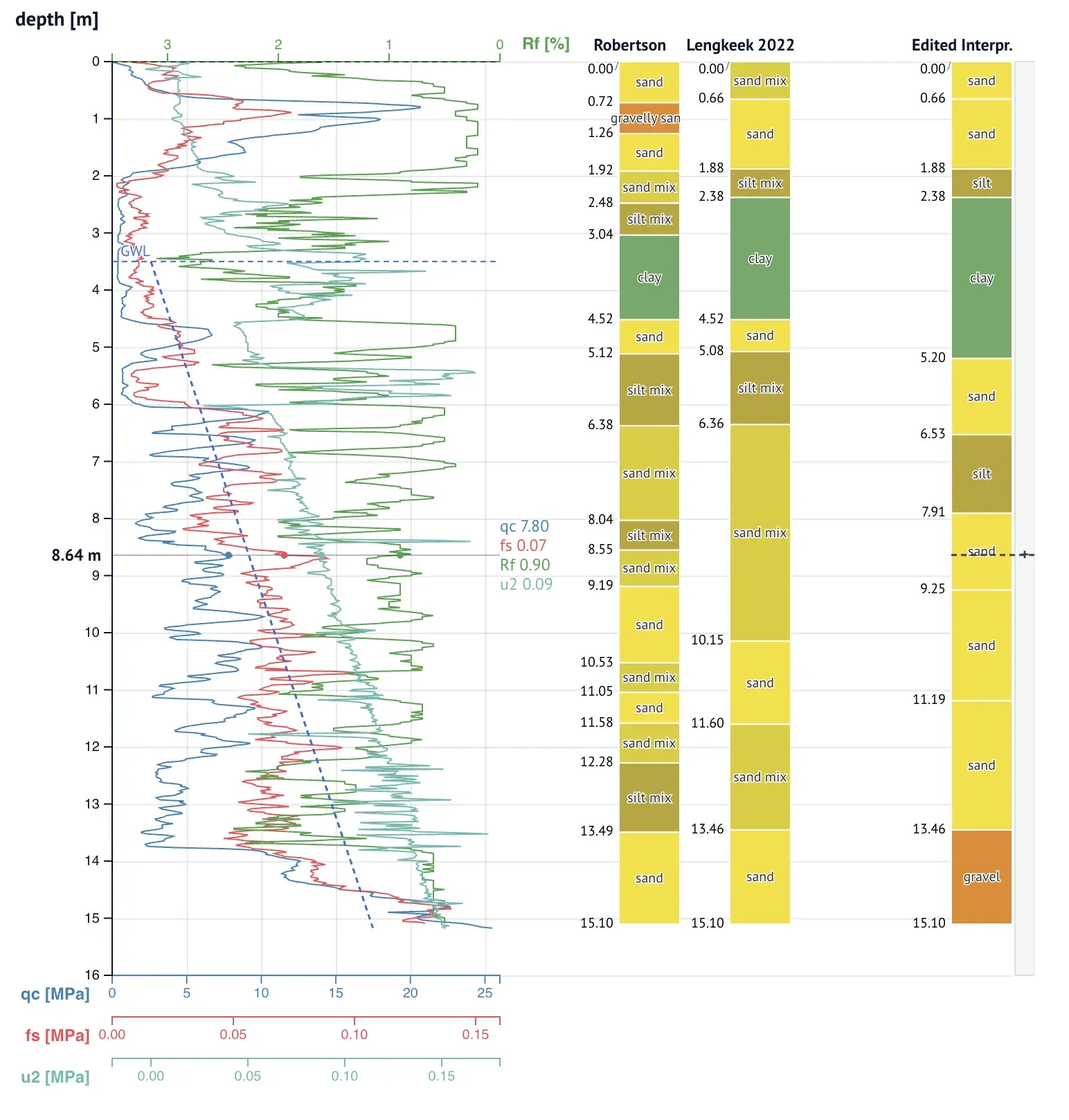
cpt-anywidget is a set of anywidget viewers for cone penetration tests (CPTs) and geotechnical borehole logs, for marimo and Jupyter notebooks. The viewers accept data from any source and share one zoomable vertical axis, showing either depth below surface or elevation in a vertical datum.
The package contains three viewers:
CPTViewershows one CPT: measurement channels, interpretation columns, a nearby borehole log, and an editable layer column.ProfileViewershows many CPTs side by side along a profile line (a cross-section).BoreholeViewershows one geotechnical borehole log with soil-composition bands.
The viewers are not tied to a national standard. The Dutch standards appear only as built-in defaults, and each has a generic counterpart:
- The BRO column names (
coneResistance,localFriction, and so on) carry display defaults; aChannelbinding does the same for any other column name. - The
"nap"key carries axis defaults for the Dutch vertical datum; aVerticalbinding does the same for any other datum. - The borehole converters color layers by BRO soil names; the
layerstrait itself takes plain dicts from any source, with your own colors.
Requirements
Section titled “Requirements”- Python 3.10 or newer.
- A notebook environment: marimo, Jupyter, or another anywidget host.
Install
Section titled “Install”Install cpt-anywidget from PyPI:
uv add cpt-anywidgetor with pip: pip install cpt-anywidget.
The package has no other dependencies beyond anywidget itself. Readers such as brodata or pygef are yours to choose and install.
Minimal example
Section titled “Minimal example”Put this code in a notebook cell:
import polars as plfrom cpt_anywidget import CPTViewer
df = pl.DataFrame({    "depth": [0.0, 0.02, 0.04],         # m below surface    "coneResistance": [0.1, 0.4, 0.9],  # MPa    "localFriction": [0.01, 0.02, 0.02],})
CPTViewer(df, vertical="depth", channels=["coneResistance", "localFriction"])
The notebook shows the widget when the cell returns it, with each channel plotted against the shared vertical axis.
Prepare the data
Section titled “Prepare the data”The data argument takes
tidy
columns: a polars or pandas DataFrame, or a dict mapping column names
to any equal-length iterables (lists, tuples, numpy arrays). Each row
is one depth sample. Each column is one measurement.
The widgets never parse file formats or convert units; that is the reader’s job, and any reader can work:
- brodata for Dutch BRO data
- pygef for GEF files and also geotechnical BRO XML files
- python-ags4 for AGS files
- plain CSV files using
polars.read_csv
Column names are free to choose. The BRO names (coneResistance,
localFriction, frictionRatio, porePressureU1, porePressureU2,
and inclination) come with built-in labels, units, and colors. For a
column with a different name, pass a Channel binding:
from cpt_anywidget import Channel
CPTViewer(df, channels=[Channel("qn", label="qn", unit="MPa", color="tomato")])
Select the vertical coordinate
Section titled “Select the vertical coordinate”Set vertical to the column that holds the vertical coordinate. A
vertical coordinate is one of two kinds:
- a depth below surface, in m, positive down
- an elevation in a vertical datum, in m, positive up: the surface elevation minus the depth
Any column can be the vertical coordinate once you bind it with a
Vertical:
from cpt_anywidget import Vertical
CPTViewer(df, vertical=Vertical("elevation", label="TAW [m]", up=True))
The names "depth" and "nap" (elevation in the Dutch datum) carry
built-in labels and formats, the same way the BRO channel names do, so
they work as plain strings.
Use the viewer
Section titled “Use the viewer”- To zoom the vertical axis, hold the Ctrl key (Cmd on macOS) and turn the mouse wheel. A trackpad or touch device pinch also zooms, without pressing any keys.
- To pan a zoomed axis, drag in the plot area.
- To zoom to a range, hold the Shift key and drag along the axis.
- To reset the zoom, double-click in the plot area.
- To read the values at a depth, move the pointer across the plot.
The mouse wheel without a modifier key scrolls the notebook, not the chart.
Next steps
Section titled “Next steps”- Edit layers: draw a layer interpretation in the widget and read it back in Python.
CPTViewerreference: all traits, including annotations, overlays, interpretations, the borehole column, and the editable layer column.ProfileViewerreference: build a cross-section from many CPTs.BoreholeViewerreference: show a borehole log from any source, with converters for BRO BHR-GT and GEF files.- Data intake reference: the
exact data contract, and the
tidyandsplithelpers.