CPTViewer

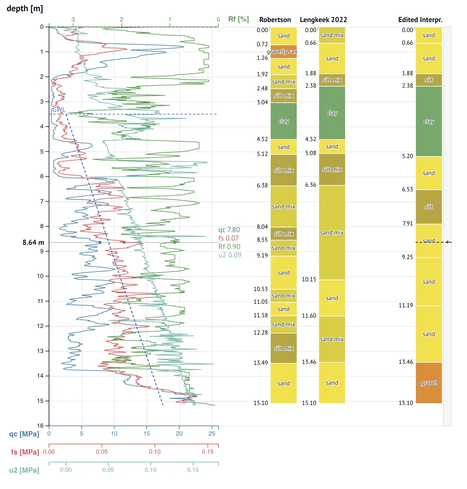
CPTViewer shows one CPT. It plots measurement channels against a shared, zoomable vertical axis. Around the plot, it can show:

• horizontal reference lines (annotations),
• polylines in a channel’s coordinates (overlays),
• read-only soil-interpretation columns,
• a nearby borehole log,
• an editable layer column that syncs edits back to Python.

from cpt_anywidget import CPTViewer, Channel

CPTViewer(
    df,
    vertical="depth",
    channels=["coneResistance", "localFriction", Channel("qn", unit="MPa")],
    limits={"coneResistance": (0, 30)},
)

Constructor

CPTViewer(data=None, *, vertical=None, channels=None, limits=None, **kwargs)

The constructor is a facade over the traits. It normalizes Python-friendly values into the JSON wire format. You can also pass any trait directly as a keyword argument. Data passed raw via cptData= skips the intake step.

Parameter	Type	Description
data	DataFrame or dict	Tidy columns: one row per depth sample, one column per measurement. Accepts a polars or pandas DataFrame, or a dict of equal-length lists. Goes through tidy: samples become JSON-safe, and rows sort into render order.
vertical	str, Vertical, or dict	The column that holds the vertical coordinate. Must be present in data. "depth" sorts ascending, "nap" descending. See Vertical.
channels	list	The channels to plot, in axis stacking order. Mix column-name strings, Channel bindings, and raw dicts.
limits	dict	{column: (min, max)} axis overrides. The vertical pair may come in either order; the constructor orients it to the render direction.
**kwargs		Trait names pass through unchanged: annotations=, interpretations=, borehole=, …

Channel

Channel binds a data column to a plotted channel. The data keeps its own column names; the binding adapts the chart. Only key is required. Omitted fields fall back to the built-in display defaults.

from cpt_anywidget import Channel

Channel("qn", label="qn", unit="MPa", color="tomato", side="bottom")

Field	Type	Description
key	str	The column name in the data. Required.
label	str	The axis label. Default: the key.
unit	str	The unit shown on the axis and in readouts.
color	str	Any CSS color. Default: a palette color.
side	str	"bottom" or "top": which side the x axis stacks on. Default: "bottom".

Built-in channel defaults

Columns with these names need no binding:

Column	Label	Unit	Side
coneResistance	qc	MPa	bottom
localFriction	fs	MPa	bottom
porePressureU1	u1	MPa	bottom
porePressureU2	u2	MPa	bottom
frictionRatio	Rf	%	top
inclination	incl	°	top

Bottom axes stack left to right. Top axes stack right to left.

Traits

The traits are the JSON wire format between Python and the browser. Every trait syncs live: set a trait on an existing widget and the chart updates.

cptData — dict

The measurement data: {"depth": [...], "coneResistance": [...], ...}. Each key is a column name. Each value is a list of samples. All lists have equal length. Use None for a missing sample — NaN is not valid JSON and breaks the sync. The first sample renders at the top.

Prefer the data constructor argument, which enforces this contract.

verticalKey — str or dict

The cptData column that is the vertical coordinate. Default: "depth". "depth" (positive down) and "nap" (positive up) carry built-in display defaults. A {"key", "label"?, "up"?, "format"?} dict binds any other column. See Vertical.

channels — list

The channels to plot, in axis stacking order. Entries are a column key or a {"key", "label"?, "unit"?, "color"?, "side"?} dict. Overrides merge over the built-in defaults. Unknown keys add new plottable channels. An empty list plots all built-in channels present in the data.

axisLimits — dict

Per-channel [min, max] axis overrides, for example {"coneResistance": [0, 30], "depth": [0, 25]}. Key the vertical override by the verticalKey. Explicit limits are honored exactly. Omitted channels fall back to the data-driven min and max.

annotations — list

Horizontal reference lines, for example a groundwater level:

[{"at": 1.2, "label": "GWL", "color": "steelblue", "dash": "4 2",
  "position": "right", "offset": [0, -4]}]

at is a value in the current vertical coordinate. position is "left", "center", or "right". offset moves the label by [dx, dy] pixels.

overlays — list

Polylines drawn in a channel’s x coordinate against the vertical axis, for example a fitted hydrostatic pore-pressure line:

[{"channel": "porePressureU2", "points": [[0.0, 1.2], [0.5, 6.0]],
  "color": "black", "dash": "2 2", "width": 1}]

points are [x, v] pairs: x in the channel’s unit, v in the current vertical coordinate. An overlay whose channel is not plotted is skipped.

interpretations — list

Read-only interpretation columns, stacked right of the plot:

[{"label": "Robertson",
  "layers": [{"top": 0.0, "bottom": 2.4, "label": "sand", "color": "#f4e04d"}]}]

top and bottom are values in the current vertical coordinate.

borehole — dict

A nearby borehole log, rendered left of the plot on the shared axis:

{"label": "BHR000000123456",
 "layers": [{"top": 1.2, "bottom": -0.8, "label": "klei",
             "bands": [{"x1": 0, "x2": 1, "color": "#78a86c", "hatch": "/"}]}]}

Each layer holds proportional soil-composition bands with x in [0, 1] and an optional matplotlib-style hatch character. An empty dict {} hides the column.

The borehole and the CPT have different surface elevations. Express both in a shared datum such as NAP — convert with to_vertical. See layers_from_bhrgt for the band shape.

editedLayers — list, bidirectional

The manually editable layer column, stacked after the interpretation columns:

[{"top": 0.0, "bottom": 2.4, "class": "sand"}]

top and bottom follow the same convention as an interpretation column. class references a soil_classes entry by name and drives the fill and the label. Explicit color and label are fallbacks for classless layers only.

The front end writes edits back to this trait. Observe it to read the user’s picks:

viewer.observe(lambda change: store(change["new"]), names="editedLayers")

In the widget, the user can:

• drag a boundary to move it,
• click in the lane beside the column to split a layer there,
• click the × near a boundary to merge two layers (the upper layer keeps its class),
• click a layer to pick its class from a pie menu.

soil_classes — list

The soil-class palette, the single source of truth for layer colors:

[{"name": "sand", "color": "#f4e04d", "label": "Sand"}]

Layers reference an entry via their class key. Override this trait to change the classes or colors project-wide.

Default

• gravel
• sand
• silt
• clay
• peat.

width, height — int

The plot size in pixels. 0 (the default) falls back to 400×800. Layer columns widen the widget beyond width.