ProfileViewer

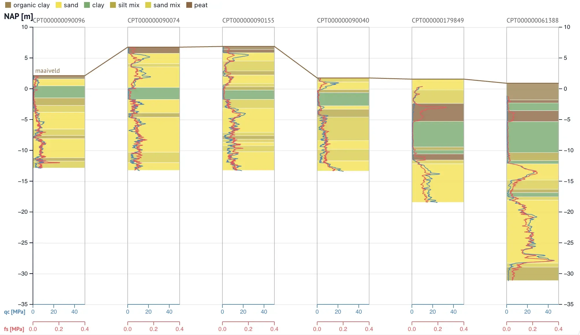
ProfileViewer shows a length profile (a cross-section): many CPTs side by side as strips on one shared, zoomable vertical axis. Each strip is anchored by its chainage along the profile line. A toolbar toggle switches between true-scale spacing and equal spacing. A click selects a strip and syncs its name back to Python.

from cpt_anywidget import ProfileViewer, chainage

positions = chainage({
    "CPT-01": (120601.0, 487429.0),   # map coordinates, in profile order
    "CPT-02": (120655.0, 487410.0),
})

ProfileViewer(long_df, positions=positions, channels=["coneResistance"])

Constructor

ProfileViewer(data=None, *, positions=None, name="name", vertical=None,
              channels=None, layers=None, limits=None, **kwargs)

The constructor is a facade over the traits. You can also pass any trait directly as a keyword argument. Data passed raw via cpts= skips the intake step.

Parameter	Type	Description
data	DataFrame or dict	Tidy long-format columns: every CPT’s samples stacked, with a name column that tells them apart. Rows are grouped per CPT via split; each group then goes through tidy.
positions	dict	{name: chainage} in m along the profile line. Every name in data must be present; a missing name raises. Omitted: input order, one unit apart — only sensible with equal spacing. See chainage.
name	str	The column that holds the CPT names. Default: "name".
vertical	str, Vertical, or dict	The vertical-coordinate column. Default: "nap" — a profile compares elevations across CPTs.
channels	list	The channels every strip plots. Mix column-name strings, Channel bindings, and raw dicts. Omitted: cone resistance only.
layers	dict	{name: [{"top", "bottom", "color"?, "label"?}, ...]} interpreted layers per CPT, drawn as a backdrop behind the strip’s curves. A name absent from data raises.
limits	dict	{column: (min, max)} axis overrides. The plotted channel’s pair sets the one scale shared by all strips.
**kwargs		Trait names pass through unchanged.

chainage

chainage(coords)

Computes the cumulative along-profile distance per CPT from map coordinates. Feed the result to ProfileViewer as positions.

Parameter	Type	Description
coords	dict	{name: (x, y)} in a projected CRS (for example RD New), in profile order.

Each CPT’s chainage is the summed straight-line distance over its predecessors. The first entry is at 0.

Traits

cpts — list

The strips:

[{"name": "CPT-01", "distance": 0.0,
  "data": {"nap": [...], "coneResistance": [...]},
  "layers": [{"top": 1.2, "bottom": -0.8, "color": "#f4e04d"}]}]

distance is the chainage in m. data follows the cptData contract. layers is optional and renders as a semi-transparent backdrop behind the strip’s curves.

verticalKey — str or dict

The data column that is the vertical coordinate. Default: "nap". Same contract as CPTViewer.verticalKey.

axisLimits — dict

[min, max] overrides. The plotted channel’s key sets the one scale shared by all strips. Key the vertical override by the verticalKey.

channels — list

The channels every strip plots, stacked axis slots in list order. Same entry shape as CPTViewer.channels. An empty list plots cone resistance only.

overlays — list

Profile-space lines over the strips. Two forms:

# a polyline in (chainage, vertical) space
[{"points": [[0.0, 1.2], [54.0, 0.8]], "label": "GWL", "color": "steelblue"}]

# per-strip levels, for example each CPT's surface elevation
[{"levels": {"CPT-01": 1.2, "CPT-02": 0.9}, "label": "surface"}]

points pairs are [distance, v]: distance in m chainage, v in the vertical coordinate. Under equal spacing, the x positions interpolate between the strip anchors.

levels draws each value flat across that strip’s width, with sloping connectors between consecutive strips. An absent name bridges to the next strip with a value. An explicit None breaks the line.

Both forms accept color, dash, and width.

annotations — list

Horizontal reference lines spanning the whole profile. Same shape as CPTViewer.annotations.

equalSpacing — bool, bidirectional

False (the default) anchors strips at true chainage. True spaces them evenly. The toolbar toggle in the widget writes this trait back.

selected — str, bidirectional

The clicked strip’s name, "" when nothing is selected. Clicking the selected strip again deselects it. Observe this trait to react in Python, for example to open a full CPTViewer beside the profile:

profile.observe(lambda change: open_cpt(change["new"]), names="selected")

stripWidth — int

Pixels per strip. 0 (the default) falls back to 90.

width, height — int

The plot size in pixels. 0 falls back to 700×500. Width is a minimum: the svg grows past it, and the widget scrolls sideways, whenever true-scale chainage or the strip count needs the room.