BoreholeViewer

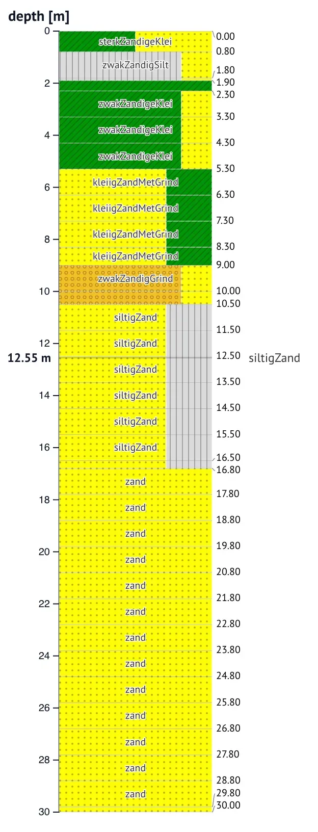
BoreholeViewer shows one geotechnical borehole log: soil-composition bands per layer on a shared, zoomable vertical axis, with hover readouts and reference-line annotations. The zoom and brush interactions match CPTViewer, so the two can sit side by side on the same axis.

from cpt_anywidget import BoreholeViewer

BoreholeViewer(layers=[
    {"top": 0.0, "bottom": 1.5, "label": "klei",
     "bands": [{"x1": 0, "x2": 1, "color": "#78a86c"}]},
])

The layers trait is plain dicts, so any source works: BRO XML, GEF, AGS, or your own interpretation. For the common Dutch formats there are converters: layers_from_bhrgt for brodata’s BRO BHR-GT objects and layers_from_bore for pygef’s borehole logs (GEF or BRO XML).

Traits

layers — list

The borehole layers, shallowest first:

[{"top": 0.0, "bottom": 1.5, "label": "klei",
  "bands": [{"x1": 0.0, "x2": 0.7, "color": "#78a86c"},
            {"x1": 0.7, "x2": 1.0, "color": "#f4e04d", "hatch": "."}]}]

top and bottom are values in the current vertical coordinate. Each layer holds proportional soil-composition bands: x1 and x2 are fractions in [0, 1]. hatch is an optional matplotlib-style pattern character (-, /, \, ., o, |) rendered as an SVG pattern.

The widget labels each layer boundary with its depth, in a strip right of the bands. When layers get thin, the labels dodge apart and leader lines point back to their boundaries — the same behavior as the interpretation columns in CPTViewer.

A layer can also carry an optional description — free text such as a field description. While you hover the layer, the soil name and the description show word-wrapped in the readout area right of the label strip.

verticalKey — str or dict

The vertical coordinate the layers are expressed in. Default: "depth". Only used for the axis label and the readout format — the layer order drives the axis direction. Same contract as CPTViewer.verticalKey.

axisLimits — dict

{verticalKey: [min, max]} override for the vertical axis. The data-driven fallback spans the first layer’s top to the last layer’s bottom.

annotations — list

Horizontal reference lines, for example a groundwater level. Same shape as CPTViewer.annotations.

width, height — int

The plot size in pixels. 0 (the default) falls back to 220×800. The boundary-label strip and the hover readouts widen the widget beyond width.

layers_from_bhrgt

layers_from_bhrgt(bhrgt, vertical_key="depth")

Converts a brodata.bhr.GeotechnicalBoreholeResearch object into the layers trait. This helper needs the bro extra (cpt-anywidget[bro]), which installs brodata.

Parameter	Type	Description
bhrgt	GeotechnicalBoreholeResearch	A parsed BRO BHR-GT object from brodata.
vertical_key	str, Vertical, or dict	The target vertical coordinate. "depth" keeps depth below surface. A positive-up coordinate such as "nap" converts through the borehole’s surface offset.

Each descriptive-log layer becomes {"top", "bottom", "label", "bands"}. The bands come from brodata’s BRO lithology table. A soil name missing from that table gets a single gray band.

from brodata.bhr import GeotechnicalBoreholeResearch
from cpt_anywidget import BoreholeViewer, layers_from_bhrgt

bhrgt = GeotechnicalBoreholeResearch("bhrgt.xml")
BoreholeViewer(layers=layers_from_bhrgt(bhrgt, "nap"), verticalKey="nap")

layers_from_bore

layers_from_bore(bore, vertical_key="depth")

Converts a pygef.bore.BoreData — pygef’s parse of a GEF or BRO XML borehole — into the layers trait. pygef normalizes both formats to BRO geotechnical soil names, so the layers get the same lithology colors and hatches as layers_from_bhrgt. A layer’s remarks (the field description) becomes its description, shown on hover. Needs pygef for parsing and the bro extra for the lithology table.

Parameter	Type	Description
bore	BoreData	A parsed borehole from pygef.read_bore.
vertical_key	str, Vertical, or dict	The target vertical coordinate, as in layers_from_bhrgt. Positive-up coordinates use the bore’s delivered vertical position offset.

import pygef
from cpt_anywidget import BoreholeViewer, layers_from_bore

bore = pygef.read_bore("borehole.gef")
BoreholeViewer(layers=layers_from_bore(bore), verticalKey="depth")